Create Census Dot Density Data in JupyterLab and HEAVY.AI
Try HeavyIQ Conversational Analytics on 400 million tweets
Download HEAVY.AI Free, a full-featured version available for use at no cost.
GET FREE LICENSE
Last week we released our newest public demonstration that takes demographic dot density maps one step further by mapping data from the 1990, 2000, 2010, and 2020 censuses, representing over a billion points at the one person to one dot resolution.
With these three decades of data and intuitive maps and charts, we ended up with a set of dashboards that allow us to explore and interrogate 30 years of US population changes at the very granular census block group level.
To best show you all the results and how we made it possible, we prepared a three-part blog series, a collection of videos, and published a public demo so you can explore your neighborhood or hometown.
This three-part blog series will show you the following:
- The first part explores some of the surprising knowledge gained from the analysis and visualizations.
- The second part (the remainder of this post) discusses how we acquired the data for each census and the Python notebooks used to turn the census block group polygons into individual points.
- The final part explores how we created the charts, maps, and dashboards in HeavyImmerse.
Let's create something extraordinary!
The challenge with getting 4 Censuses
Like BigQuery or AWS, most public data providers only carry the recent 2010 decennial census and a few years of ACS data from the last decade. For most geospatial projects, this is all that's needed. ACS only goes back to 2005. Trying to compare three decades of census data is unusual, and there is no one provider of data that provides easy access to block group level from 1990 to 2020 (that we could find).
2000 and 2010 Censuses
We started writing code to create dots with the easiest-to-find census data (2000 and 2010). For these, we used the Summary File 1 (SF 1) Census API endpoint. The hardest part of using this API is figuring out the correct variables to request. As long as you know the appropriate fields (e.g., P004005), it's relatively easy to get the correct data for each state.
The next step is joining the demographic data to the census block group geometries. These shapefiles were available within the census FTP directory (in the Tiger Lines directory).

For the 2000 and 2010 censuses, this loop worked well for getting the census block group demographics and geometry.
1990 Data Acquisition
The 1990 SF1 block group endpoint is currently down, so we went to the National Historical Geographic Information System (NHGIS) to get the 1990 data. Their data downloading process is pretty straightforward. You need to download the demographic and geometry data separately and join on the aptly named GISJOIN key.

2020 Data Acquisition
In August 2021, the Public Law 94-171 redistricting data was released for the 2020 census. These files come in an odd .PL file format that is challenging to work within most tools.
Thankfully, different groups like the Redistricting Data Hub have converted these data into Shapefiles and CSVs. These files include the demographic fields and geometries, so huge thanks to the Redistricting Hub for providing this.

Functions for Creating Points From Polygons
After acquiring the data for the four censuses, the next step was to create the dot density points. We used Geopandas, Shapely, and some functions from Andrew Gaidus' Census Mapping post to do this.
These are the core functions:
The overall gist of these functions is to take a polygon, an integer for the population count for that block group, and the number of people per point (e.g., 25 people for 1 point). The function runs a while loop that creates random points (using Numpy's RandomState) within the polygon's maximum and minimum x and y bounds. It then uses Geopandas' .within method to test whether that point falls within the polygon or not. If it does, it adds them to the array of points.
To make this clearer, let's look at an example census block group. Here's a block group in the Mission Neighborhood in San Francisco, CA.

The function would take the polygon geometry of the block group, the integer 1550, and the number of people per point (e.g., 1 or 25) to create the dot density points for the white population.
It would then run the while loop, randomly creating points, testing if they fall within the polygon boundaries, and adding them to an array/list of points.
After the point creation and while loop finish, it creates 123 points for the number of black people who live in that block group, and so on.
The points are then pushed up into an HEAVY.AI table using PyOmniSci's method load_table_columnar. We ran these functions to create 1 point for every person, approximately 1.1 billion points across the four censuses. No other geospatial platform is capable of working with this much data natively.
The result is a table with points that look like this:

Challenges and Pitfalls
There were a few challenges we encountered getting the data and transforming it.
API Fields
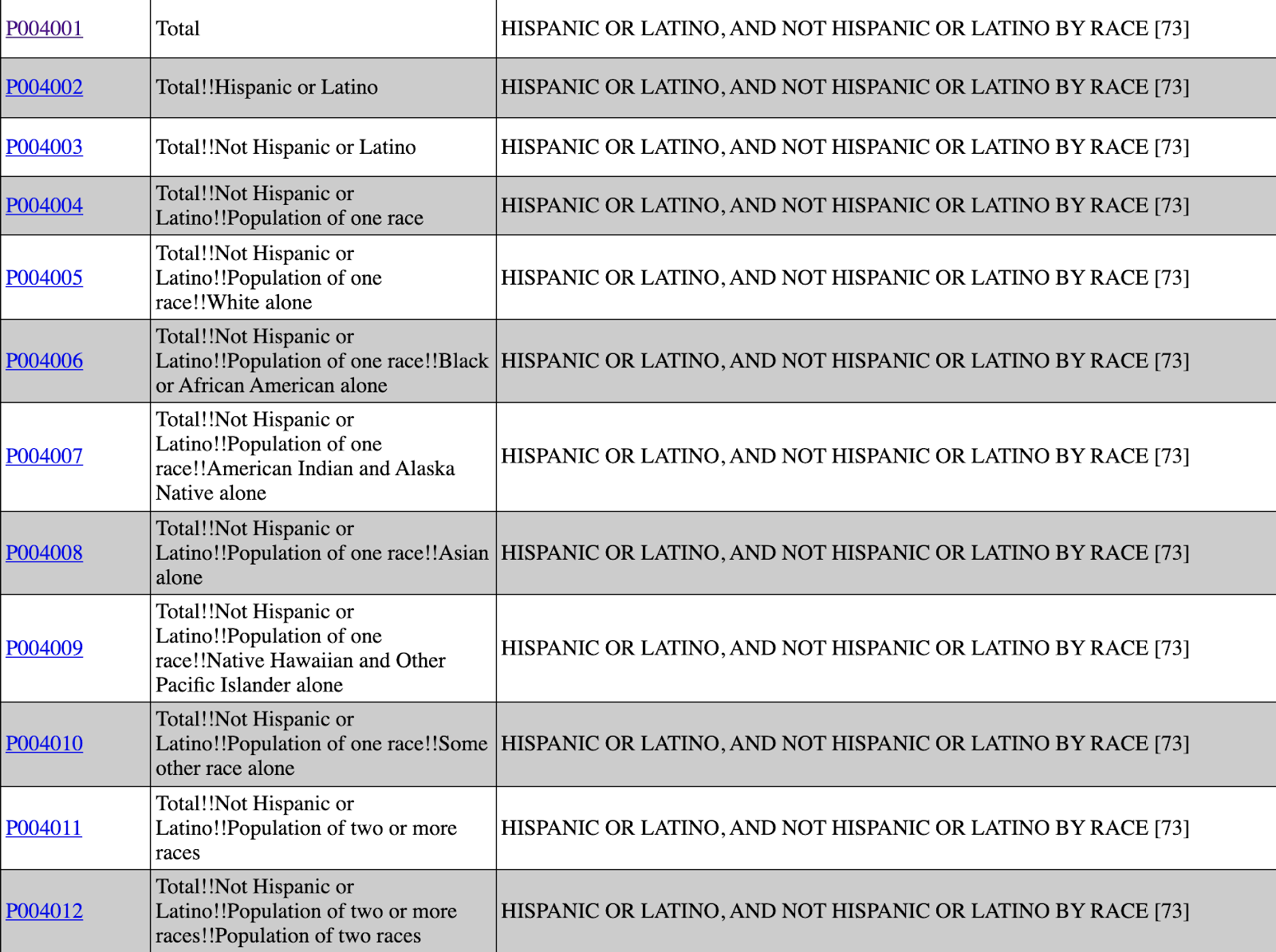
It was sometimes challenging to know the right demographics field to go for in the data. The fields are hard to parse (P005003 vs. P005004) visually and can change subtly from one census to another. The other major challenge with ethnicity fields is using the non-hispanic population count fields vs. the default value. For example, in the 2010 census, you need to use the Total!!Not Hispanic or Latino!! Fields like these:

Whereas you might think you need to use these:

This distinction is confusing because someone can be White, Black, or another race and Hispanic. If you use those latter fields, you end up with a total count greater than the actual population for the block group. This was confusing and frustrating, at first, to end up with 400M+ points (more than the US population) created for the 2010 census.
Here it's worth calling out the challenge of oversimplifying 300+ million people's ethnicities into just a few categories. Americans are an increasingly multi-racial and mixed-race society, and pushing everything into six ethnic categories oversimplifies things a bit.
Someone could be both Hispanic and white or from the Caribbean and East Indian, so which color should their point be? This is one of the challenges with dot density mapping, as there are only so many point colors you can include without making the map unusable.
Memory and Timeouts
Another challenge was working with such a large amount of data in a notebook (tens of millions of points for some states) and not running out of memory. When pushing the data up to HEAVY.AI, we split the giant data frame into smaller chunks with the following code.
Numpy RandomState
The other challenge we ran into was creating random points using the NumPy RandomState. The original functions had the RandomState object in the while block, making duplicate points for each ethnicity (which stacked points on top of one another). Once we moved it above the functions, the points created were truly random across all ethnicities.
Differing Coordinate Reference Systems
The 1990 Census geometries were in the North America Albers Equal Area Conic CRS. Thankfully, Geopandas was able to convert them to WGS 84 using the to_crs method easily.
Long Data Processing Times
Creating hundreds of millions of points takes quite a while. A notebook will sometimes timeout or crash when it is left running that long. A notebook isn't the right tool to use for that much data. The workaround was to convert the notebooks to standard python scripts and run them on a Linux server using the Tmux library. This keeps the code running after you've closed the terminal. A better solution might be to use PySpark or something similar to parallelize the code.
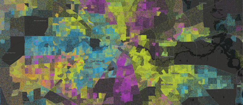
Explore the data for yourself here!
And while you are at it check our method to process the census data and create the points in these notebooks:
We'd love to hear about your findings once you've used the dashboard, as well as any feedback you may have. Please share those thoughts and experiences with us on LinkedIn, Twitter, or our Community Forums!