
Taming Data to Tackle Cyber-Threats with OmniSci
Try HeavyIQ Conversational Analytics on 400 million tweets
Download HEAVY.AI Free, a full-featured version available for use at no cost.
GET FREE LICENSENOTE: OMNISCI IS NOW HEAVY.AI
In February 2020, Gartner published a cyber risk assessment report titled “The Urgency to Treat Cybersecurity as a Business Decision” where Gartner senior analyst Paul Proctor explained various critical trends within the cybersecurity side of business, where companies are being forced to cope with emerging threats in an environment increasingly defined by challenges like government regulation, societal perception and the COVID-19 pandemic. The most common risk to a network’s security is an intrusion which could be in form of a brute force attack, denial of service, or even an infiltration from within a network. So, to prevent these scenarios from affecting the organization, we generally have an Intrusion Detection System (IDS) or Host-Based Intrusion Detection System (HIDS) installed. The installed IDS or HIDS systems monitor network traffic for suspicious activities and these systems issue alerts or take pre-defined actions in case of such identified issues.
Let's take a real-world example: the recent, massive DDoS attack on AWS infrastructure using CLDAP Reflection (connection-less Lightweight Directory Access Protocol reflection) as mentioned here from AWS. This technique relies on vulnerable third-party CLDAP servers and amplifies the amount of data sent to the victim’s IP address by 56 to 70 times and with that amount it was bombarding packets at around 2.3 TB per second. While the disruption caused by the AWS DDoS Attack was far less severe than it could have been, the sheer scale of the attack and the implications for AWS hosting customers potentially losing revenue and suffering brand damage were significant. And Intrusion Detection Systems (IDS) are precisely present to prevent the above scenario from affecting the organization.
There are many commercial offerings and open-source tools which when configured well can find anomalies in firewall traffic based on some static rules, or the so-called signatures. These signatures are constructed and updated multiple times a day so that they could detect these known anomalies or unusual traffic patterns. But generally, a rule-based system can detect only known anomalies, and as it is known from the past behaviors, the attack patterns change and evolve, and new patterns appear. So, a rule-based system can’t detect such altered attacks. This is where intelligent machine learning-based systems come into play.
OmniSci Accelerated Analytics
To understand and address these kinds of problems, cybersecurity professionals would first want to quickly explore, visualize and analyze a large amount of data to identify network patterns and possibly create rules based on what they find. This quickly surfaces the classic problem for any data scientist during the feature engineering phase or the data preparation phase where they are not able to use the entire dataset and have to work with a subset of the data using the ML tools and libraries of their choice. But OmniSci is different. It is fast, even on the largest datasets, and tightly integrated with the most popular machine learning platforms and libraries like Jupyter, Pandas, IBIS, and RAPIDS. With OmniSci, the data scientist has access to their entire dataset, queried in familiar tools at unprecedented speed, as well as access to advanced computation resources to play with the data and evaluate models faster.
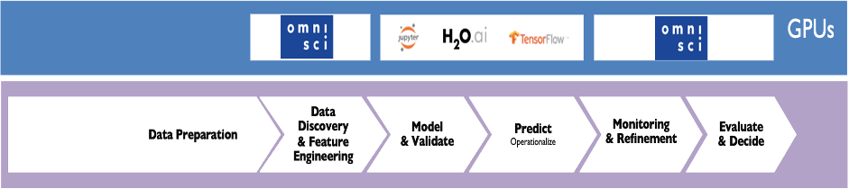
It is also important to articulate and translate the predictions made by the trained model, for evaluation and decision. The OmniSci platform is able to visualize the end-to-end ML pipeline for a better understanding of the situation. Let’s look more specifically at each step of this workflow.
Explore the Data
The most important aspect of any analytics platform is how quickly one can explore and mine the data with an interactive experience and speed-of-thought visualization. And this becomes very important in case of a cybersecurity use case due to the nature of the data which are data generated at high velocity and high volume. To achieve this, we can explore the data with OmniSci Immerse. OmniSci Immerse not only reduces the time to insights, it dramatically expands a security analyst's ability to find previously hidden correlations. A powerful combination of features, working seamlessly with the server-side power of OmniSciDB and Rendering engine, results in an immersive, unbound visual analytics and dashboarding experience. Analysts and data scientists can interact with conventional charts and data tables, as well as massive-scale scatterplots and geo charts created by OmniSci’s GPU-enabled renderer. For this demo, we have collected sample data from our internal firewall at OmniSci and loaded it into the OmniSci platform. Below is the screengrab from the Immerse dashboard where we have created various charts based on the firewall data.

Let’s first look at some numbers from the image above. We can see that this dataset has almost around 1.3 Billion records with data transactions happening on our network from over 237 countries, with around 6 million source IPs and 1.4 million destination IPs and an average packet size of around 87 Bytes. One other important data point is the Firewall action taken chart, which defines what percentage of data packets were allowed and how many were blocked based on the defined static rules. In our case, we have almost 17% of our packets blocked. This feature would also be used as our dependent variable or label in our machine learning task.
We’ve seen that 70-80% of cyber data has a spatial component to it. And data analysis which includes geospatial data is becoming far more common – it’s not treated as a separate discipline with separate tools like it often was in the past. In this dashboard, we also have the data representation for all the connections plotted on a point map which provides us an overall view of all the traffic onto our network. Apart from this we also have the port and related protocols used in these connections in the bar chart with connections from the city details table.

We also have plotted against time on the action taken by the firewall based on the packet length or data length with details on the requested address and top source IPs. And we’ve included a heatmap with the number of hits on our firewall distributed across weekdays. And looking at this it’s pretty clear that almost every weekday we have a high number of records ranging from around 10 million to 15 million connections per hour.
Now after going through all the charts let’s do a quick analysis of an event or pattern and find out various details like which IP, from which region, and which protocol has caused this event. Let’s also look at the average packet length based on the actions chart.

We start by browsing through the Firewall Action | Average packet length chart to zoom in to the anomalies and explore and analyze data and events at that particular time to gather more information and take relevant action. All of the data exploration and visualization is happening on the entire corpus of data rather than a subset of it and with massive acceleration supported by OmniSciDB and server-side rendering on GPUs. With this we can drill down to a specific event interactively, and use what we find to create a new rule for blocking similar addresses or traffic patterns.
After going through the wonderful visual experience of the raw data from the Firewall on Immerse, now let’s move the focus to add machine learning capabilities to this data. We’ll start with data cleaning and feature engineering to prepare it to be consumed by various algorithms. Feature engineering is all about creating new input features from your existing ones. So, data cleaning is a process of subtraction whereas feature engineering is a process of addition. With OmniSci Immerse we not only can explore and analyze data, but with the tight integration with Jupyter, data scientists can jump directly to their notebooks from the Immerse screen, and get access to the entire dataset on OmniSci.

The data scientists now can not only work on the data but also present the outcomes of each stage back to Immerse for visualization. For example, in the below image 6, we have charts detailing the feature and model selection steps.

Feature selection (also known as subset selection) is a process commonly used in machine learning, wherein subsets of the features available from the data are selected for the application of a learning algorithm. The best subset contains the least number of dimensions that most contribute to accuracy; and we discard the remaining, unimportant dimensions. So here in this first chart, we are looking at the correlation table. Data correlation is a way to understand the relationship between multiple variables and attributes in our dataset. So, if we see the feature heatmap here we can evaluate how each feature is related to the other. All the features are placed in the X and Y axis and depending on the derived correlation values we can understand the relationship.
For instance, in the charts above, we can see that our dataset has perfectly positive or negative attributes, and therefore, there is a high chance that the performance of the model will be impacted by a problem called multicollinearity. The easiest way to solve this problem is to delete or eliminate one of the perfectly correlated features. Next, we look at other ways and means of feature selection like the Recursive Feature Elimination method. In the dashboard image below we have used different algorithms to find the suitable features, including comparing Random Forest and Extratreeclassifier as well as other popular ones like XGBoost. Based on the outputs as seen in these charts the algorithms have selected the best suitable features for model training. The header length looks to be the most important feature for XGBoost while longitude is the most important for Extratreeclassifier and TTL for Random Forest.
After fixing on the features let’s see and identify which could be the best suitable model now to train and test with these selected features.

In this chart, we have selected multiple models for training and looked at various model performance parameters to choose the right model for our data. Only looking at model accuracy might not choose the most accurate ML model. Parameters like F1 score, accuracy, precision, and recall have been plotted here. And based on the details we can easily find out that the tree-based ensemble models like Random Forest and XGBoost have performed better.
But apart from accuracy or F1 score or AUC, we also need to look at another important aspect of model performance, which is speed to train and infer as well as log loss. By looking at these charts we can see that KNN took the largest amount of time to train and score while again the tree-based models have a better output. The last chart shows the log-loss of each model. Based on these charts, the tree-based classifiers have performed better, and based on these details, we selected and used XGBoost as our choice of algorithm for classifying connections as good or bad (and there should be allowed or blocked).
Based on our data exploration and model selection criteria we selected the XGBoost classifier model to train on our firewall dataset. For this, we selected 70% of our firewall data to train the model and the rest 30% of the data to test the model. The answer we are trying to solve here is to check if a connection based on various features needs to be blocked or allowed to pass through without looking at any static rule which has been defined manually.

The output from our model after testing has an AUC-ROC value of perfect 1, and the confusion matrix shows the various model decisions. We have chosen the AUC-ROC measure because we understand that the accuracy of the model is based on specific cut-points or thresholds, whereas AUC tells us something about how well the model separates the two classes, no matter where the threshold value is. In short, for the ROC curve, the higher it is, the better the model could be. Also, the confusion matrix in this chart here describes the performance of our XGB classification model (or "classifier") on the test data for which the true values were known.
Here we have a trained model with some great scores. The logical end for this would be to take this model to production for inferencing on near real-time streaming logs. And while the model is in production we might need to compare the model predictions versus the firewall actions.

So if we look at this dashboard above, we are visually articulating our model decisions and actual firewall decisions by first selecting all packets blocked by the firewall and then selecting packets which the model predicted to be safe. With these, we can visually compare the results (if there were false alarms by the firewall or where the model needs further improvement) on billions of rows of data with a real-time capability.
To conclude the post, we saw how, with a combination of the OmniSci advanced analytics platform and modern ML techniques, we can not only help cybersecurity professionals to quickly visualize and analyze large datasets, but also integrate machine learning methods to build a modifiable, reproducible, and extensible solution to learn and tackle sophisticated attackers who can easily bypass basic IDS or HIDS systems. Learn more about our Data Science Platform today.
Watch the full demo below: